Week 14 Lab: ArbExtras.jl

The goal of this lab is to familiarize yourself a little bit with the Julia package ArbExtras.jl. From the README of the package we have

This package extends Arblib with some methods for enclosing roots, enclosing extrema and computing integrals.

The package started development during my PhD with the goal to give reusable implementations of algorithms that were used in my research. The type of methods that are implemented and which type of input they are optimized for has been heavily influenced by the projects that I worked on during that time.

There is no separate documentation for this package, so instead take some time to read through the README. The functions we will take a look at during this lab are:

1. isolate_roots(f, a::Arf, b::Arf): Used for isolating all roots of

a function $f$ on the interval $[a, b]$.

1. refine_root(f, root::Arb): Used to refine an already existing

enclosure $root$ of a function function $f$.

1. extrema_enclosure(f, a::Arf, b::Arf): Used for enclosing the

extrema of a function $f$ on an interval $[a, b]$.

The first two are closely related to what we talked about during Week 7, in particular Lecture 2.

Isolating roots

In Week 7 Lecture 2 we looked at isolating the roots of the function $f(x) = \sin(5x) - 5x + x^2 + 4$. We will redo that with the isolate_roots function from ArbExtras. Let us start by loading the required packages and defining the function.

using Arblib, ArbExtras, Plots
setprecision(Arb, 128)

f(x) = sin(5x) - 5x + x^2 + 4

f (generic function with 1 method)

Plotting the function, we have

plot!(range(0, 5, 1000), f)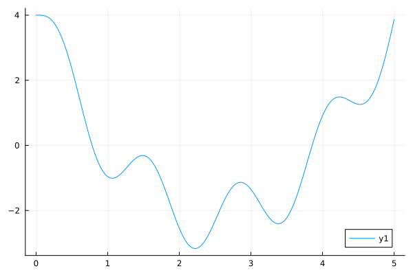

We can isolate all the roots of this function on the interval $[0, 5]$ with

roots, flags = ArbExtras.isolate_roots(f, Arf(0), Arf(5))

(Tuple{Arblib.Arf, Arblib.Arf}[(0.625, 0.9375), (3.75, 4.0625)], Bool[1, 1])

TASKS:

• Read the documentation of ArbExtras.isolate_roots (you can access the documentation by typing ? in the Julia REPL and writing ArbExtras.isolate_roots).
• What do the return values roots and flags mean?
• How many functions does $f$ have on the interval $[0, 5]$?
• Run the function with verbose = true, i.e. roots, flags = ArbExtras.isolate_roots(f, Arf(0), Arf(5), verbose = true). What output do you see?

You can experiment with other functions and intervals. For example you can look at:

• What happens if there is a zero on the boundary? For example for $f(x) = 2 - x + \sin(\pi x)$ on the interval $[0, 2]$. What happens if you extend the interval to $[0, 3]$?
• What happens for double roots? For example $f(x) = x^2$ on the interval $[-1, 2]$.

Refine roots

In Week 7 Lecture 2 we also looked at refining roots of functions. Among other things we talked about the interval Newton method. The refine_root function implements this method.

Let us consider the function $g(x) = e^x - 4x$, which has a root on the interval $[0, 1]$. We can refine this root with

g(x) = exp(x) - 4x
ArbExtras.refine_root(x -> exp(x) - 4x, Arb((0, 1)))

[0.35740295618138890306881110405590475332 +/- 9.26e-39]

TASKS:

• Read the documentation of ArbExtras.refine_root.
• Run the function with verbose = true, i.e. ArbExtras.refine_root(x -> exp(x) - 4x, Arb((0, 1))). What output do you see?
• Run the function with the input interval $[-1, 0]$ (where there is not root). What happens?
• If you increase the precision using setprecision(Arb, P) for some P (say 1024), how does the enclosure change? What does the verbose = true output look like?

Enclose extrema

The function ArbExtras.extrema_enclosure can be used to enclose the extrema of a function on an interval. Let us consider the function $h(x) = x\sin(x) + x\cos(2x)$ on the interval $[0, 10]$. We can enclose the extrema with

h(x) = x * sin(x) + x * cos(2x)
ArbExtras.extrema_enclosure(h, Arf(0), Arf(10))

([-9.50835044063309514253 +/- 5.97e-21], [10.3367982489424558454 +/- 4.93e-20])

TASKS:

• Read the documentation of ArbExtras.extrema_enclosure (it is quite long).
• Run the function with verbose = true. What output do you see?
• Add the argument rtol = 1e-5. How does the result change? If you also run it with verbose = true, how does the output change?
• Change the function to maximum_enclosure and minimum_enclosure. How do these differ?
• Run the maximum_enclosure function with the argument ubound_tol = 20. What do you get? This can be useful if you only need to prove that the function is bounded by some value, but don't need to get a tight enclosure of the maximum.